As the final part of my project I was then asked to look at a more challenging situation – the mixing of a jet entering normal to a main flow, of the kind illustrated below.
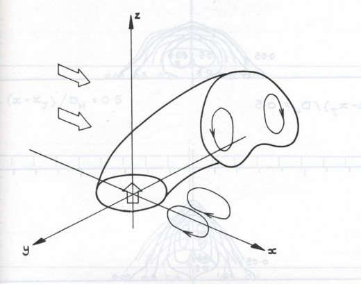
Jet Entering Normal to a Main Flow
This class of flows was chosen for study because it occurs in a number of practical problems of (then) high interest – the one we most had in mind was the dilution region of a cylindrical or (even closer) annular gas turbine combustor.
Plus, it was a way of exploring the range of validity of our parabolic computational method. We were aware that, for cases where the jet velocity was as large as, or larger than, the main flow velocity, the flow would certainly be elliptic, with (among other elliptic features) some flow reversal just behind the jet entry. However, for lower jet velocities, there was the expectation/hope that a parabolic method would yield reasonable results, much more economically that a full elliptic approach. So it was a sort of “stress test” of the parabolic approach!
Specifically, the situation that I considered was a rectangular passage, with, part way down the passage, a square side jet entering normally at the centre of one of the long passage sides – as shown below.
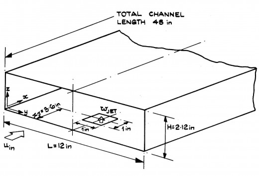
The Configuration Computed and Measured (apologies for the non-SI units!)
As well as performing computations (using the SIMPLE-based solution method described earlier, with the “standard“ k-epsilon model), I also undertook a short experimental study of the configuration shown.
We looked at turbulent flow conditions, with jet velocity/main flow velocity ratios of 0.1 and 0.3 – in the expectation that these would be low enough for the parabolic approach to work.
The results were “interesting” to say the least! The computed flow fields were very different from the measurements, even for gross characteristics of the flow, such as the jet trajectory. While the measurements showed the jet essentially attaching itself to the near wall, the predictions showed the jet spreading out across the channel, and eventually reaching the far wall.
So – not a good result! Not a very positive note on which to complete my PhD work!
Of course, in research, a negative result is not necessarily a failure – so long as it contributes to a better understanding of the phenomena in question. In this case the conclusion was that, even for the modest jet/main flow velocity ratios we considered, the flow was in fact more “elliptic” than we had expected. Specifically, the measurements showed significant lateral variation in pressure across the passage in the region immediately downstream of the jet – in conflict with the third requirement cited earlier for the flow to be truly parabolic. It seemed likely that the effects of this wrong assumption in my parabolic computations had led to the observed errors in the solutions.
This led to the recognition that there are flows (such as this one) for which, while the first two requirements for parabolic flow are valid (or close enough), the third (relatively small lateral pressure variation) is not valid. Spalding identified these as an intermediate class of flows, between parabolic and elliptic, which he named initially “Semi-Elliptic” and then “Partially Parabolic”.
The point about these is that they can be solved more economically that “fully elliptic” flows, by a sort of composite method. The flow is treated as parabolic, except that the local (rather than mean) pressure gradient is used in the main-flow momentum equation. This means that the pressure has to be stored 3D – while other variables can be stored 2D. Solution is obtained by a marching integration sweep, as for a parabolic flow – but at the end of each complete sweep through the solution domain, the 3D pressure field is corrected (using a form of SIMPLE), and the solution sweep is then repeated using the new pressures. This is repeated until convergence.
There are two advantages over a “fully-elliptic” solution – convergence is obtained faster (because the iteration sweep exploits the essentially one-way character of the flow), and there is a much reduced storage requirement (because only pressure is solved 3D).
A method of this kind was developed by one of Spalding’s students, Pratap, soon after I completed my research, and was applied successfully to a range of practical situations, including my transverse jet case, and flows in curved pipes and passages. The method was then used, alongside SIMPLE-based parabolic and elliptic methods, at Imperial College and at CHAM, until the advent of the PHOENICS general-purpose CFD software in 1981.
This study completed my PhD project – which had encompassed the development of 3D boundary-layer computational methods, their successful application to a range of laminar and turbulent channel flows, and, finally, an exploration of the limitations of the parabolic, boundary-layer approach for certain classes of flows. Quite enough it seemed to me – and also, fortunately, to David Gosman, my PhD supervisor!
So, in the autumn of 1972 I joined CHAM, the commercial CFD operation then just beginning at Imperial College. More on this – the birth of commercial CFD – in future blogs …